RL:model free

当模型太大，无法通过迭代得到最佳策略，我们就需要使用model free RL

Model-free prediction

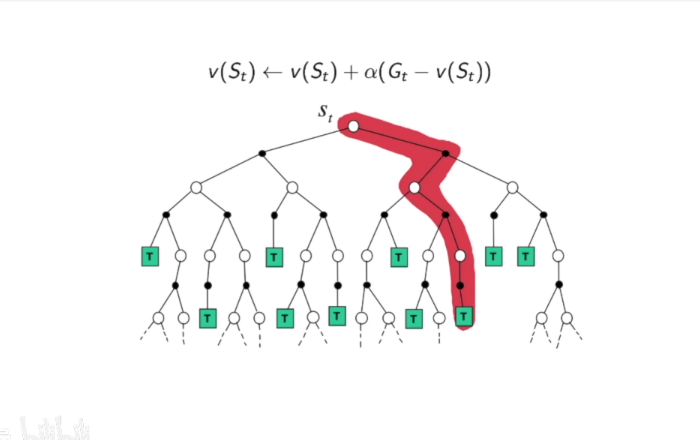
Monre Carlo policy evaluation

• Return: $Gt=R{t+1}＋\gamma R{t+2}+\gamma^2R{t+3}+…$underpolicy$\pi$
• $v^{\pi }(s)=E_{\tau -\pi }[G_t|s_t=s]$, thus expectation over trajectories $\tau$Tgenerated by following $\pi$
• MC simulation: we can simply sample a lot of trajectories, computethe actual returns for all the trajectories, then average them
• MC policy evaluation uses empirical mean return instead of expectedreturn
• MC does not require MDP dynamics/rewards,no bootstrapping,anddoes not assume state is Markov.
• Only applied to episodic MDPs (each episode terminates)

算法流程

To evaluate state v(s)

• Every time-step t that state s is visited in an episode,
• Increment counter $N(s)\to N(s)＋1$
• Increment total return $S(s)\to S(s)+G_t$
• Value is estimated by mean return $v(s)=s(s)/N(s)$By law of large numbers,$v(s)\to v^{\pi }(s)$as$N(s)\to \mathrm{\infty }$

蒙特卡洛的核心思想是通过多次迭代，取每个状态value的均值

• Collect one episode (S1,A1,R1,…. St)
• For each state st with computed return Gt$$\begin{gathered} N(S_t)=N(S_t)+1 \\ v(S_t)=v(S_t)+\frac{1}{N(S_t)}(G_t-v(S_t)) \end{gathered}$$
• Or use a running mean (old episodes are forgotten). Good fornon-stationary problems.$$v(S_t)=v(S_t)+\alpha (G_t-v(S_t))$$

$\alpha$在这里可以看做学习率

Temporal Diffenence learning

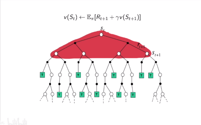
• Objective: learn $v_{\pi }$ online from experience under policy $\pi$
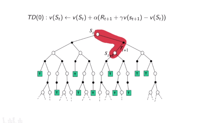
• Simplest TD algorithm: TD(0)
  • Update $v(St)$towardestimatedretur$R{t+1}+~v(St+1)$

$$v(S_t)=v(S_t)+\alpha (R_{t+1}＋\gamma v(S_t+1)-v(S_t))$$

• $R{t+1}+\gamma v(S{t+1})$ is called TD target
• $t=R_{t+1}+\gamma v(S_t+1)-v(S_t)$ is called the TD error
• Comparison: Incremental Monte-Carlo
  • Update $v(S_t)$ toward actual return $G_t$ given an episode i$$v(S_t)=v(S_t)+\alpha (G_t-v(S_t))$$我们也使用可以n步的TD

Difference Between TD and MC

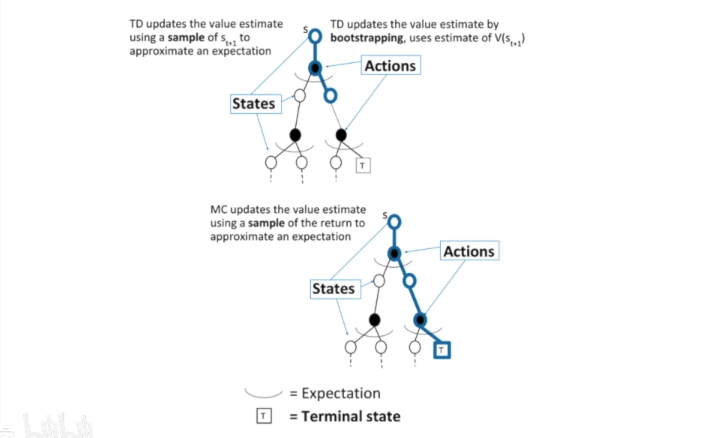
TD可以随时进行学习，MC只有在走完决策树后才能学习

• DP

• MC
  
• TD
  

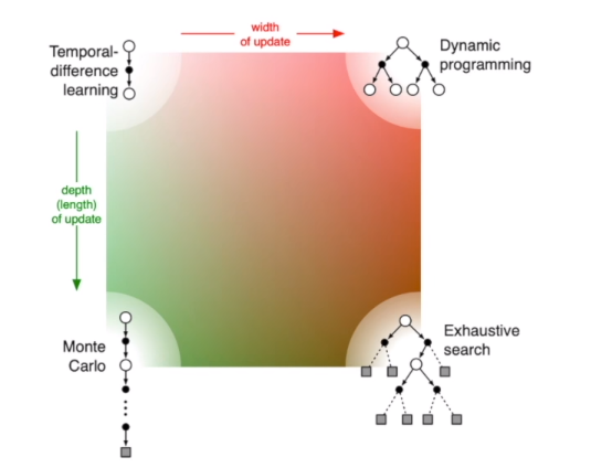
Model free control

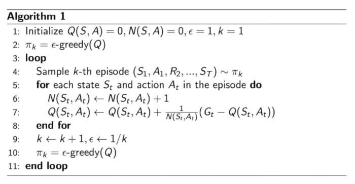
Monte Carlo with $ϵ$greedy Exploration

• Trade-off between exploration and exploitation (we will talk aboutthis in later lecture)
• $ϵ$Greedy Exploration: Ensuring continual exploration
  • All actions are tried with non-zero probability
  • With probability 1 - $ϵ$ choose the greedy action
  • With probability $ϵ$choose an action at random

$$\pi (a|s)=\{\begin{array}{ll}ϵ/|A|+1-ϵ& a=argma{x}_{a\in A}Q(s,a\\ ϵ/|A|& otherwise\end{array}$$

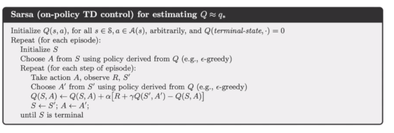
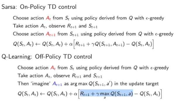
Sarsa:On-Policy TD Control

• An episode consists of an alternating sequence of states andstate-action pairs:

• $ϵ$-greedy policy for one step, then bootstrap the action value function:

$$Q(S_t,A_t)=Q(S_t,A_t)+\alpha [R_{t+1}+Q(S_{t+1},A_{t+1})-Q(s_t,A_t)]$$

• The update is done after every transition from a nonterminal state $S_t$
• TD target $\phit= R{t+1}+Q(S{t+1},A{t+1})$

On policy Learning off-policy Learning

• On-policy learning: Learn about policy $\pi$ from the experiencecollected from $\pi$
  • Behave non-optimally in order to explore all actions, then reduce the
    exploration $ϵ$-greedy
• Another important approach is off-policy learning which essentiallyuses two different polices:
  • the one which is being learned about and becomes the optimal policy
  • the other one which is more exploratory and is used to generate
    trajectories
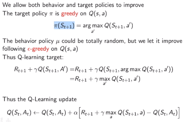
• Off-policy learning: Learn about policy $\pi$ from the experience sampledfrom another policy $\pi$
  • $\pi$: target policy
  • $\mu$: behavior policy

off policy 会选择更加激进的策略，通过激进策略的反馈优化target policy

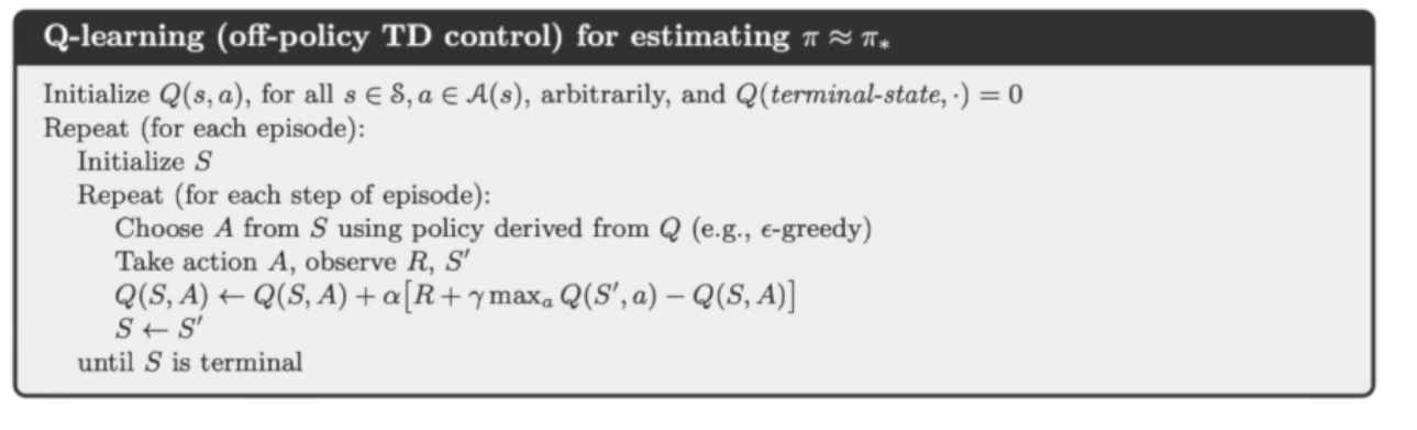
Off policy control with Q-Learning